Curriculum and Pedagogy

useR 2025

Elijah Meyer & Maria Tackett

Curriculum

Curriculum guidelines

Use technology to explore concepts and analyze data. (GAISE, 2016)
Incorporate software/apps to explore concepts and work with data. (GAISE revision, in progress)
All programs should (a) expose students to technology tools for reproducibility, collaboration, database query, data acquisition, data curation, and data storage; (b) require students to develop fluency in at least one programming language used in data science and encourage learning a second language. (Two-Year College Data Science Summit, 2018)
The two pillars of computational and statistical thinking should not be taught separately…both should be present for the most effective and efficient teaching. (Curriculum Guidelines for Undergraduate Programs in Data Science, 2014)

Intro Data Science

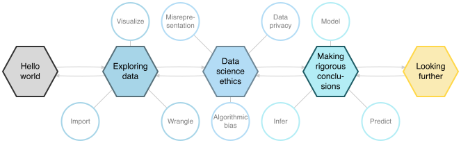
Image from Data Science in a Box

Intro Data Science topics

Unit 1: Exploring data

Data visualization
Exploring multivariable relationships
Data wrangling
Importing data

Unit 2: Making rigorous conclusions

Relationships between multiple variables
Predicting numeric and binary outcomes
Model building and feature engineering
Model evaluation and cross validation
Simulation-based inference

Intro Data Science topics

Additional topics (varies by instructor)

Interactive dashboards with Shiny
Working productively with AI tools
Text analysis
Customizing Quarto reports and presentations

Computing throughout course

Statistical analysis using R
Reproducible reports using Quarto
Version control and collaboration using git and GitHub

Computing as a learning objective

“The goal of teaching computing and information technologies is to remove obstacles to engagement with a problem.”

(Nolan & Temple Lang, 2010)

Students gain experience using professional computing tools
Students develop reproducible workflow while learning statistical methods
Students gain experience working with more complex and realistic data
Students develop computational thinking and build confidence to handle computational challenges

Pedagogy

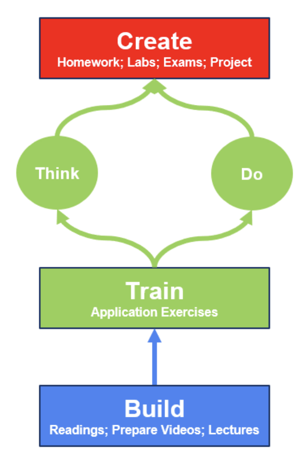
Build: Introduce new content
Train: Put concepts into practice through hands-on class activities
- Do: Steps needed to accomplish a task
- Think: How to accomplish task in future
Create: Demonstrate learning through a variety of assessments

Source: Meyer and Çetinkaya-Rundel (2025, preprint)

Tidyverse

The tidyverse is an opinionated collection of R packages designed for data science. All packages share an underlying design philosophy, grammar, and data structures.

-tidyverse.org

library(tidyverse)

Tidyverse in data science workflow

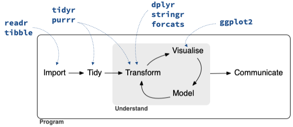
Source: Çetinkaya-Rundel et al. (2022)

Pedagogical benefits of the tidyverse

Consistency: Syntax, function interfaces, argument names and order follow patterns
Mixability: Ability to use base R and other functions within tidyverse syntax
Scalability: Unified approach that works for data sets from a wide range of types and sizes
User-centered design: Function interfaces designed with users in mind
Readability: Interfaces designed to produce readable code
Community: Large, active, and welcoming community of users and resources
Transferability: Data manipulation verbs inherit SQL’s query syntax

Source: Çetinkaya-Rundel et al. (2022)

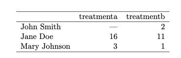
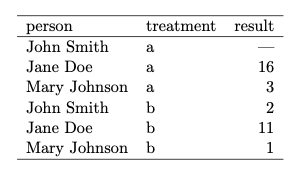
Tidy data

Each variable forms a column.
Each observation forms a row.
Each type of observational unit forms a table.

Not tidy data

Tidy data

The pipe

The pipe, |>, is used to pass information from one function to another in the tidyverse.

When reading code aloud in English, say “and then” whenever you see a pipe. Below is a pipeline for a children’s poem.*

Little bunny Foo Foo
Went hopping through the forest
Scooping up the field mice
And bopping them on the head

foo_foo |>
  hop(through = forest) |>
  scoop(up = field_mice) |>
  bop(on = head)

Data: Palmer penguins

We will analyze the penguins data set from the palmerpenguins R package maintained by Dr. Allison Horst. This data set contains measurements and other characteristics for penguins observed near Palmer Station in Antarctica. The data were originally collected by Dr. Kristen Gorman.

We will use the following variables:

species: a factor denoting penguin species (Adélie, Chinstrap and Gentoo)
flipper_length_mm: an integer denoting flipper length (millimeters)
body_mass_g: an integer denoting body mass (grams)

Click here for the full codebook.

`penguins` data frame

library(palmerpenguins)
penguins

# A tibble: 342 × 8
   species island    bill_length_mm bill_depth_mm flipper_length_mm body_mass_g sex     year
   <fct>   <fct>              <dbl>         <dbl>             <int>       <int> <fct>  <int>
 1 Adelie  Torgersen           39.1          18.7               181        3750 male    2007
 2 Adelie  Torgersen           39.5          17.4               186        3800 female  2007
 3 Adelie  Torgersen           40.3          18                 195        3250 female  2007
 4 Adelie  Torgersen           36.7          19.3               193        3450 female  2007
 5 Adelie  Torgersen           39.3          20.6               190        3650 male    2007
 6 Adelie  Torgersen           38.9          17.8               181        3625 female  2007
 7 Adelie  Torgersen           39.2          19.6               195        4675 male    2007
 8 Adelie  Torgersen           34.1          18.1               193        3475 <NA>    2007
 9 Adelie  Torgersen           42            20.2               190        4250 <NA>    2007
10 Adelie  Torgersen           37.8          17.1               186        3300 <NA>    2007
# ℹ 332 more rows

Base R: Compute summary statistics

Compute the mean flipper length for Palmer penguins.

mean(penguins$flipper_length_mm)

[1] 200.9152

Base R: Compute summary statistics

For each species, compute the number of penguins and the mean flipper length. Display the results in descending order by number of penguins.

Compute number of penguins by species

num_penguins <- aggregate(flipper_length_mm ~ species, data = penguins, FUN = length)
names(num_penguins)[2] <- "num_penguins"

Compute mean flipper length by species

mean_flipper <- aggregate(flipper_length_mm ~ species, data = penguins, FUN = mean)
names(mean_flipper)[2] <- "mean_flipper_length"

Base R: Compute summary statistics

For each species, compute the number of penguins and the mean flipper length. Display the results in descending order by number of penguins.

Combine results and sort data frame

df <- merge(num_penguins, mean_flipper)
df[order(df$num_penguins, decreasing = TRUE), ]

    species num_penguins mean_flipper_length
1    Adelie          151            189.9536
3    Gentoo          123            217.1870
2 Chinstrap           68            195.8235

Base R: Full code

num_penguins <- aggregate(flipper_length_mm ~ species, data = penguins, FUN = length)
names(num_penguins)[2] <- "num_penguins"

mean_flipper <- aggregate(flipper_length_mm ~ species, data = penguins, FUN = mean)
names(mean_flipper)[2] <- "mean_flipper_length"

df <- merge(num_penguins, mean_flipper)
df[order(df$num_penguins, decreasing = TRUE), ]

    species num_penguins mean_flipper_length
1    Adelie          151            189.9536
3    Gentoo          123            217.1870
2 Chinstrap           68            195.8235

Your turn!

Use tidyverse syntax to make the data frame described below:

For each species, compute the number of penguins and the mean flipper length. Display the results in descending order by number of penguins.

Tip

See dplyr reference for list of functions.

Closer look at the code

For each species, compute the number of penguins and the mean flipper length. Display the results in descending order by number of penguins.

penguins

# A tibble: 342 × 8
   species island    bill_length_mm bill_depth_mm flipper_length_mm body_mass_g sex     year
   <fct>   <fct>              <dbl>         <dbl>             <int>       <int> <fct>  <int>
 1 Adelie  Torgersen           39.1          18.7               181        3750 male    2007
 2 Adelie  Torgersen           39.5          17.4               186        3800 female  2007
 3 Adelie  Torgersen           40.3          18                 195        3250 female  2007
 4 Adelie  Torgersen           36.7          19.3               193        3450 female  2007
 5 Adelie  Torgersen           39.3          20.6               190        3650 male    2007
 6 Adelie  Torgersen           38.9          17.8               181        3625 female  2007
 7 Adelie  Torgersen           39.2          19.6               195        4675 male    2007
 8 Adelie  Torgersen           34.1          18.1               193        3475 <NA>    2007
 9 Adelie  Torgersen           42            20.2               190        4250 <NA>    2007
10 Adelie  Torgersen           37.8          17.1               186        3300 <NA>    2007
# ℹ 332 more rows

Closer look at the code

For each species, compute the number of penguins and the mean flipper length. Display the results in descending order by number of penguins.

penguins |>
  group_by(species)

# A tibble: 342 × 8
# Groups:   species [3]
   species island    bill_length_mm bill_depth_mm flipper_length_mm body_mass_g sex     year
   <fct>   <fct>              <dbl>         <dbl>             <int>       <int> <fct>  <int>
 1 Adelie  Torgersen           39.1          18.7               181        3750 male    2007
 2 Adelie  Torgersen           39.5          17.4               186        3800 female  2007
 3 Adelie  Torgersen           40.3          18                 195        3250 female  2007
 4 Adelie  Torgersen           36.7          19.3               193        3450 female  2007
 5 Adelie  Torgersen           39.3          20.6               190        3650 male    2007
 6 Adelie  Torgersen           38.9          17.8               181        3625 female  2007
 7 Adelie  Torgersen           39.2          19.6               195        4675 male    2007
 8 Adelie  Torgersen           34.1          18.1               193        3475 <NA>    2007
 9 Adelie  Torgersen           42            20.2               190        4250 <NA>    2007
10 Adelie  Torgersen           37.8          17.1               186        3300 <NA>    2007
# ℹ 332 more rows

Closer look at the code

For each species, compute the number of penguins and the mean flipper length. Display the results in descending order by number of penguins.

penguins |>
  group_by(species) |>
  summarise(n = n(), 
            )

# A tibble: 3 × 2
  species       n
  <fct>     <int>
1 Adelie      151
2 Chinstrap    68
3 Gentoo      123

Closer look at the code

For each species, compute the number of penguins and the mean flipper length. Display the results in descending order by number of penguins.

penguins |>
  group_by(species) |>
  summarise(n = n(), 
            mean = mean(flipper_length_mm)
            )

# A tibble: 3 × 3
  species       n  mean
  <fct>     <int> <dbl>
1 Adelie      151  190.
2 Chinstrap    68  196.
3 Gentoo      123  217.

Closer look at the code

For each species, compute the number of penguins and the mean flipper length. Display the results in descending order by number of penguins.

penguins |>
  group_by(species) |>
  summarise(n = n(), 
            mean = mean(flipper_length_mm)
            ) |>
  arrange(desc(n))

# A tibble: 3 × 3
  species       n  mean
  <fct>     <int> <dbl>
1 Adelie      151  190.
2 Gentoo      123  217.
3 Chinstrap    68  196.

Your turn! [Time permitting]

Create a new data frame that only contains the penguin from each species with the largest body mass.
Use dplyr functions to continue exploring the penguins data set.

“The tidyverse provides an effective and efficient pathway for undergraduate students at all levels and majors to gain computational skills and thinking needed throughout the data science cycle.”

-Çetinkaya-Rundel et al. (2022)

What about AI?

We recommend minimal use of generative artificial intelligence (AI) for coding when coding proficiency is a learning objective in an introductory course
There are a variety of perspectives on using generative AI tools to teaching coding:
- Bien, J., & Mukherjee, G. (2025). Generative AI for Data Science 101: Coding Without Learning To Code. Journal of Statistics and Data Science Education, 33(2), 129-142.
- Generative AI in Statistics and Data Science Education (Journal of Statistics and Data Science collection)
- Leveraging LLMs for student feedback in introductory data science courses by Mine Çetinkaya-Rundel (USCOTS presentation)
- Learning the tidyverse with the help of AI tools by Mine Çetinkaya-Rundel (Tidyverse blog)

Infrastructure

RStudio in the cloud

Removes the most common hurdle to get started with computing - installation and configuration
- Start using R on Day 1!
Actively engage students with all aspects of the course, not just in a computing lab
Install R and RStudio on a server and provide access to students:
- Centralized RStudio Server / Posit Workbench
- Dockerized RStudio Server (what we’re using today)
- Posit Cloud

RStudio in a Docker container

RStudio in Docker containers built and maintained by Duke Office of Information Technology
Customize the pre-installed packages, data sets, etc. for your course
Students access their instance of RStudio using institution credentials

Demo

Open RStudio docker container (see email for URL)
Click File -> New File -> Quarto Document to make a new Quarto document
Parts of a Quarto document:
- YAML
- Narrative
- Code
Use Quarto for reproducible in-class activities and assignments

Discussion

What is something you’ve seen thus far that you find exciting? Want to learn more about? Would like to incorporate in your teaching?
Any other questions/ comments/ discussion points?

Curriculum and Pedagogy

Curriculum

Curriculum guidelines

Intro Data Science

Intro Data Science topics

Intro Data Science topics

Computing as a learning objective

Pedagogy

Pedagogy

Tidyverse

Tidyverse in data science workflow

Pedagogical benefits of the tidyverse

Tidy data

The pipe

Data: Palmer penguins

penguins data frame

Base R: Compute summary statistics

Base R: Compute summary statistics

Base R: Compute summary statistics

Base R: Full code

Your turn!

Closer look at the code

Closer look at the code

Closer look at the code

Closer look at the code

Closer look at the code

Your turn! [Time permitting]

What about AI?

Infrastructure

RStudio in the cloud

RStudio in a Docker container

Demo

Discussion

`penguins` data frame